BackJanuary 2026

High Fidelity 3-Dimensional Heat Diffusion

Tools

Python
NumPy
Matplotlib
MATLAB

Hardware

M1 MacBook Air (2020), 8 GB

Overview

A three-dimensional transient heat diffusion model of an EV battery module, solved with the same finite difference scheme in Python and in MATLAB on the same laptop. Both converge to the same temperature field in under 11,800 iterations. MATLAB gets there in about 81 seconds; Python takes about 3,450.

Background

Partial differential equations (PDEs) form the mathematical foundation of many models used in science, engineering, and applied technology. They describe how physical quantities evolve in space and time and are central to the analysis of systems governed by conservation laws, field interactions, and transport phenomena.

In electromagnetics, Maxwell’s equations govern the propagation of electromagnetic waves and underpin modern communication systems, including wireless data transmission and sensing technologies. In fluid mechanics and heat transfer, the Navier–Stokes equations describe the motion of fluids and the transport of thermal energy, enabling the modeling of atmospheric dynamics, thermal systems, and energy conversion processes.

Beyond individual applications, PDEs provide a unifying mathematical framework for modeling a wide range of physical phenomena, including heat diffusion, wave propagation, mass transport, acoustic transmission, and seismic activity. Their ability to capture spatially distributed behavior makes them indispensable for predicting system performance and guiding engineering design decisions.

Analytical Solutions

Analytical solutions are the gold standard in PDE analysis, as they provide exact, closed-form descriptions of a system’s behavior. When available, such solutions enable precise predictions and facilitate theoretical insight into the underlying physical processes. However, analytical solutions exist only for a limited class of problems.

In certain cases, exact solutions can be derived for well-posed PDEs with simplified geometries and boundary conditions. Classic examples include Laplace’s equation and Poisson’s equation, which arise in electrostatics, gravitation, and steady-state heat conduction. Additionally, wave phenomena are commonly described by the wave equation,

\nabla^2 \phi = 0, \qquad \nabla^2 \phi = f(x, y, z)

\frac{\partial^2 u}{\partial t^2} = c^2 \nabla^2 u

whose analytical solutions characterize the propagation of sound, light, and mechanical vibrations. In one spatial dimension, D’Alembert’s solution expresses the general solution to the wave equation as a superposition of traveling waves,

u(x, t) = f(x - ct) + g(x + ct)

These analytical formulations provide valuable insight into physical behavior such as field distributions, energy transport, and oscillatory motion.

Despite their theoretical importance, analytical solutions are often unattainable for real-world engineering systems. Complex geometries, nonlinear material properties, and coupled boundary conditions frequently preclude closed-form solutions. As a result, numerical methods play a central role in practical PDE analysis by enabling approximate solutions for systems that cannot be solved analytically.

Numerical Solutions

Analytical solutions provide exact, closed-form expressions for partial differential equations, but many engineering problems involve complex geometries, nonlinearities, or boundary conditions that render such solutions intractable. In these cases, numerical methods provide a practical framework for approximating the solution of PDEs to a desired level of accuracy.

Consider a general time-dependent partial differential equation of the form

\frac{\partial u(\mathbf{x}, t)}{\partial t} = \mathcal{L}\big(u(\mathbf{x}, t)\big) + f(\mathbf{x}, t)

where $u(\mathbf{x}, t)$ represents the state variable of interest, $\mathcal{L}$ is a spatial differential operator, and $f(\mathbf{x}, t)$ is a source term. Numerical solution techniques approximate this continuous problem by discretizing the spatial domain into a finite set of grid points or elements and, for transient problems, discretizing time into finite increments.

Spatial discretization replaces continuous derivatives with finite difference, finite volume, or finite element approximations. For example, a second-order central difference approximation of a second spatial derivative in one dimension is given by

\frac{\partial^2 u}{\partial x^2} \approx \frac{u_{i+1} - 2u_i + u_{i-1}}{\Delta x^2}

Time integration is performed by advancing the solution in discrete time steps using explicit, implicit, or semi-implicit schemes. A representative explicit time-stepping formulation can be written as

u_i^{n+1} = u_i^{n} + \Delta t\, \mathcal{L}_h\!\left(u_i^{n}\right) + \Delta t\, f_i^{n}

where $n$ denotes the time index, $\Delta t$ is the time step size, and $\mathcal{L}_h$ represents the discrete spatial operator. Common time-integration schemes include the forward Euler, backward Euler, and Crank–Nicolson methods, each offering different trade-offs between stability, accuracy, and computational cost.

To obtain a well-posed numerical problem, appropriate initial and boundary conditions are required. An initial condition specifies the state of the system at $t = 0$ , while boundary conditions constrain the solution at the spatial domain boundaries, typically in the form of Dirichlet, Neumann, or Robin conditions. The numerical solution proceeds iteratively until convergence criteria, such as bounded changes between successive time steps, are satisfied.

Although numerical solutions are inherently approximate, their accuracy can be systematically improved through mesh refinement, reduced time step sizes, and higher-order discretization schemes. These improvements increase computational cost and may introduce stability constraints. For diffusion-dominated problems, the time step is often limited by a condition of the form

\Delta t \le C\, \frac{\Delta x^2}{\alpha}

where $C$ is a stability constant and $\alpha$ is the diffusion coefficient. Consequently, the selection of discretization strategies and numerical solvers plays a central role in balancing accuracy, stability, and computational efficiency in practical PDE-based engineering simulations.

Simulation Tools

The development of numerical methods for solving partial differential equations has been significantly shaped by the growth of open-source scientific computing ecosystems. Open-source frameworks provide accessible, extensible implementations of advanced numerical techniques, enabling researchers and engineers to focus on problem formulation and analysis rather than low-level solver development. This has improved reproducibility, collaboration, and the practical adoption of PDE-based simulation across engineering disciplines.

Libraries such as FEniCS, DUNE, deal.II, and PETSc offer robust support for finite element and finite volume methods, scalable linear solvers, and parallel computation. High-level programming languages including Python, R, and Julia further lower the barrier to entry by providing expressive syntax and extensive numerical libraries for discretization, linear algebra, and visualization. These environments support rapid prototyping and exploratory analysis, while performance-critical components are often delegated to optimized backend libraries written in compiled languages such as C++ or Fortran.

Recent advances in computational assistance tools have also influenced numerical simulation workflows. Symbolic computation platforms and large language models can assist with code generation, debugging, and access to reference implementations, reducing development overhead. While such tools do not replace numerical expertise, they can complement traditional workflows by accelerating implementation and iteration in PDE-based modeling tasks.

The Benchmark

Practical engineering analysis increasingly relies on numerical simulation to study systems that do not admit analytical solutions. As a result, effective use of modern computational tools requires familiarity with numerical libraries, solver ecosystems, and visualization workflows rather than detailed knowledge of language syntax alone. Emphasis is therefore placed on selecting appropriate numerical frameworks, validating results, and understanding performance trade-offs across different software environments.

To evaluate the feasibility of conducting nontrivial PDE-based simulations on consumer hardware, this study benchmarks a representative transient heat diffusion problem using two widely adopted computational environments: an open-source workflow implemented in Python and a proprietary platform implemented in MATLAB. The comparison is designed to assess end-to-end simulation performance under identical physical assumptions, numerical methods, and hardware constraints, rather than isolated algorithmic optimizations.

The Battery Problem

Electric vehicle battery systems provide a relevant and demanding test case for numerical simulation due to the strong coupling between thermal behavior, performance, and degradation. Elevated operating temperatures accelerate aging mechanisms and reduce usable capacity, making thermal management a critical design consideration. As summarized in Table 1, battery replacement and recycling costs often represent a substantial fraction of total vehicle value, reinforcing the economic importance of predictive thermal modeling.

The simulation focuses on transient heat diffusion within a simplified battery geometry subject to representative boundary conditions. This formulation captures the dominant thermal dynamics while remaining computationally tractable, enabling a controlled comparison of numerical performance across software platforms. The problem therefore serves both as a realistic engineering application and as a benchmark for evaluating numerical simulation capability on standard laptop hardware.

BATTERY	LIFESPAN (YR)	REPLACEMENT (USD)	RECYCLING (USD)
Lithium-ion (average)	10–20	6,500–20,000+	6,500–20,000+
Nissan LEAF (30 kWh)	8–12	3,500–4,500	3,500–4,500
Nissan LEAF (40 kWh)	8–12	6,500–7,500	6,500–7,500
Chevrolet Bolt	8–12	15,000–16,000+	15,000–16,000+
Tesla Model S	10–20	12,000–20,000+	12,000–20,000+
BMW i3	8–12	13,000–15,000+	1,300–1,500+
Toyota Prius (hybrid)	10–15	2,500–4,000	250–400

Table 1. Electric vehicle battery lifespan, replacement, and recycling costs.

The Model

Figure 1 illustrates the geometry of the lithium-ion battery pack and the associated thermal boundary conditions used in this study. The configuration represents a simplified battery module with active cooling applied at the base and convective heat transfer to the surrounding environment. This formulation captures the dominant thermal transport mechanisms while remaining computationally tractable.

Figure 1. The module as modelled, to scale: a block generating heat internally, held at the coolant plate's temperature on its base and cooled by air on every other face.

The thermal behavior of the battery is modeled using the three-dimensional transient heat diffusion equation with internal heat generation,

\frac{\partial T}{\partial t} = \alpha \left( \frac{\partial^2 T}{\partial x^2} + \frac{\partial^2 T}{\partial y^2} + \frac{\partial^2 T}{\partial z^2} \right) + \frac{\dot{q}}{\rho c_p}

where $T(x,y,z,t)$ denotes the temperature field, $\alpha$ is the thermal diffusivity of the battery material, $\dot{q}$ is the volumetric heat generation rate, $\rho$ is the material density, and $c_p$ is the specific heat capacity. This formulation accounts for both conductive heat transport within the battery and internally generated heat arising from electrochemical processes.

Thermal interaction with the environment is represented through a combination of prescribed and convective boundary conditions. At the bottom surface, a linearly varying temperature profile is imposed to model coolant flow, with the temperature increasing from an inlet value $T_{\text{inlet}}$ to an outlet value $T_{\text{outlet}}$ along the height of the battery.

The remaining surfaces (top, sides, front, and back) are subject to convective heat transfer governed by Newton’s law of cooling. The resulting heat flux is proportional to the temperature difference between the battery surface and the ambient environment at temperature $T_{\text{amb}}$ , with the convective heat transfer coefficient $h_{\text{air}}$ characterizing the efficiency of heat removal.

Numerical Method

The governing equation and boundary conditions are solved numerically using a finite difference formulation. Second-order central difference schemes are employed for spatial derivatives in all three dimensions, while time integration is performed using the Crank–Nicolson method, selected for its favorable stability and accuracy characteristics in transient diffusion problems.

A non-uniform spatial mesh is used, with refined grid spacing near boundary regions where higher temperature gradients are expected. The time step is chosen to satisfy the Courant–Friedrichs–Lewy (CFL) condition in all spatial directions, ensuring numerical stability of the solution.

Parameters

The simulation is advanced in time until convergence is achieved, defined as the maximum absolute temperature difference between successive time steps falling below a prescribed tolerance. Computational progress is monitored by recording CPU time and the maximum temperature within the battery at regular intervals, ensuring both numerical stability and physical consistency of the solution.

PARAMETER	SYMBOL	VALUE	UNITS	DESCRIPTION
Battery density	$\rho$	2500	$\mathrm{kg\,m^{-3}}$	Density of the battery material
Battery specific heat	$c_p$	780	$\mathrm{J\,kg^{-1}\,K^{-1}}$	Specific heat capacity of the battery material
Battery thermal conductivity	$k$	1.5	$\mathrm{W\,m^{-1}\,K^{-1}}$	Thermal conductivity of the battery material
Thermal diffusivity	$\alpha$	$7.69\times10^{-7}$	$\mathrm{m^2\,s^{-1}}$	Calculated as $\alpha = k / \rho c_p$
Coolant inlet temperature	$T_{\text{inlet}}$	293.15	$\mathrm{K}$	Coolant entering the cooling system
Coolant outlet temperature	$T_{\text{outlet}}$	303.15	$\mathrm{K}$	Coolant leaving the cooling system
Ambient temperature	$T_{\text{amb}}$	298.15	$\mathrm{K}$	Air surrounding the battery
Coolant heat transfer coefficient	$h_{\text{coolant}}$	1500	$\mathrm{W\,m^{-2}\,K^{-1}}$	Between the battery and the coolant
Air heat transfer coefficient	$h_{\text{air}}$	10	$\mathrm{W\,m^{-2}\,K^{-1}}$	Between the battery and ambient air
Heat generation rate (base)	$\dot{q}_{\text{base}}$	10,000	$\mathrm{W\,m^{-3}}$	Base volumetric heat generation
Heat generation rate (peak)	$\dot{q}_{\text{peak}}$	25,000	$\mathrm{W\,m^{-3}}$	Peak of the sinusoidal variation

Table 2. Physical and thermal parameters used in the three-dimensional transient heat diffusion model.

Table 2 summarizes the physical and thermal parameters used in the three-dimensional finite difference simulation. Material properties, including density, specific heat capacity, and thermal conductivity, govern internal heat diffusion within the battery, while convective heat transfer coefficients characterize thermal exchange with the coolant and ambient air. The thermal diffusivity is computed from these material properties as

\alpha = \frac{k}{\rho c_p}

Internal heat generation is modeled using a sinusoidal profile to represent a simplified charge–discharge cycle, incorporating both base and peak volumetric heat generation rates.

Boundary Conditions

The initial and boundary conditions are summarized in Table 3. The battery is initialized at a uniform temperature of 25 °C. Cooling is applied at the bottom surface via a linearly varying temperature profile between the coolant inlet and outlet, while the remaining faces exchange heat with the ambient environment through convective boundary conditions. This combination captures the dominant thermal interactions relevant to battery cooling while maintaining model simplicity.

CONDITION	FACE	EXPRESSION	TEMP (°C)
Initial	All	$T(x,y,z,0)=T_{\text{initial}}$	25
Boundary	Bottom (z = 0)	$T(x,y,0,t)=T_{\text{inlet}}+(T_{\text{outlet}}-T_{\text{inlet}})\,\frac{y}{H}$	20–30
Boundary	Top (z = D)	$-k\,\frac{\partial T}{\partial z}=h_{\text{air}}(T-T_{\text{amb}})$	25 (ambient)
Boundary	Front (y = 0)	$-k\,\frac{\partial T}{\partial y}=h_{\text{air}}(T-T_{\text{amb}})$	25 (ambient)
Boundary	Back (y = H)	$-k\,\frac{\partial T}{\partial y}=h_{\text{air}}(T-T_{\text{amb}})$	25 (ambient)
Boundary	Left (x = 0)	$-k\,\frac{\partial T}{\partial x}=h_{\text{air}}(T-T_{\text{amb}})$	25 (ambient)
Boundary	Right (x = L)	$-k\,\frac{\partial T}{\partial x}=h_{\text{air}}(T-T_{\text{amb}})$	25 (ambient)

Table 3. Initial and boundary conditions applied to the three-dimensional transient heat diffusion model.

Mesh and Hardware

The battery geometry is modeled as a rectangular prism with dimensions 0.254 m × 0.1524 m × 0.1016 m in the $x$ , $y$ , and $z$ directions, respectively. To resolve expected temperature gradients efficiently, non-uniform meshes are employed in all three spatial dimensions, with refined grid spacing near boundaries subject to strong thermal fluxes.

The spatial discretization consists of 100 × 50 × 25 grid points in the $x$ -, $y$ -, and $z$ -directions, with increased resolution near the coolant interface and convective surfaces. This strategy balances numerical accuracy with computational efficiency by concentrating resolution in regions of high thermal gradient.

All simulations are executed on an Apple Silicon M1 MacBook Air (2020) with 8 GB of RAM, providing a representative consumer-grade hardware platform for performance evaluation.

Results

Both implementations ran the same problem on the same mesh, to the same tolerance, on the same laptop. They agree on the answer and differ by more than an order of magnitude in how long it takes.

SOLVER	ITERATIONS	RUNTIME	RELATIVE
Python	11,760	~3,450 s	1×
MATLAB	11,762	~81 s	~40×

Table 4. The same problem, mesh, and tolerance on the same laptop.

Python

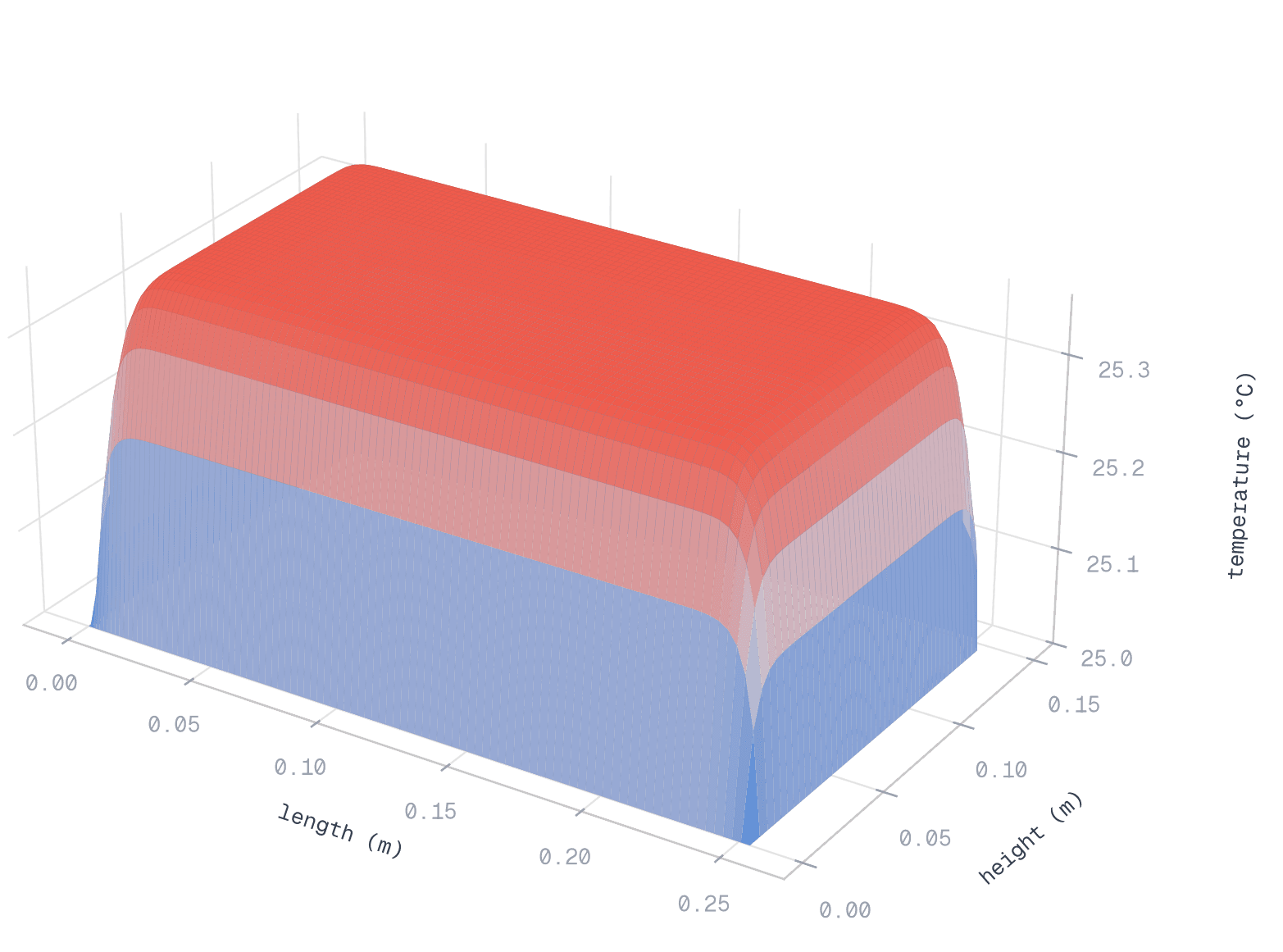
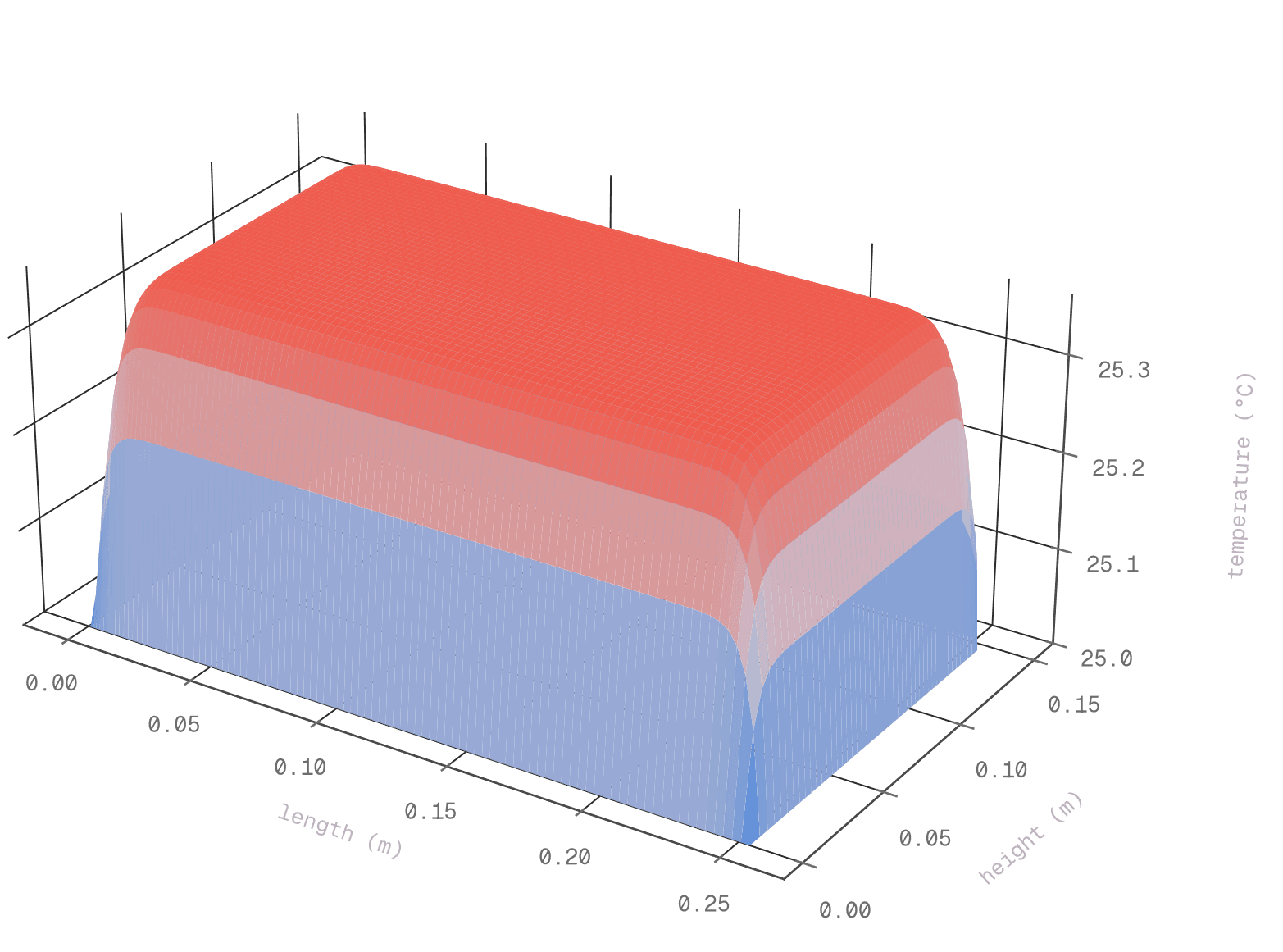
The Python implementation converged after 11,760 iterations, indicating attainment of a steady-state temperature distribution under the specified convergence criterion. The total CPU time was approximately 3,450 seconds, reflecting the computational cost of solving a three-dimensional transient heat diffusion problem with a refined, non-uniform mesh on consumer-grade hardware.

The resulting temperature field at mid-depth of the battery exhibits a clear vertical gradient, with elevated temperatures near the upper region of the domain. This behavior is consistent with internal heat generation combined with convective boundary conditions applied to the exposed surfaces. The spatial distribution confirms that the numerical solution captures the expected thermal trends within the battery geometry.

Surface plot of temperature across the battery's length and height at mid-depth: a flat plateau near 25.35 °C falling steeply to 25.0 °C at the edges — Figure 2. Steady-state temperature at mid-depth of the battery, from the Python solver.

MATLAB

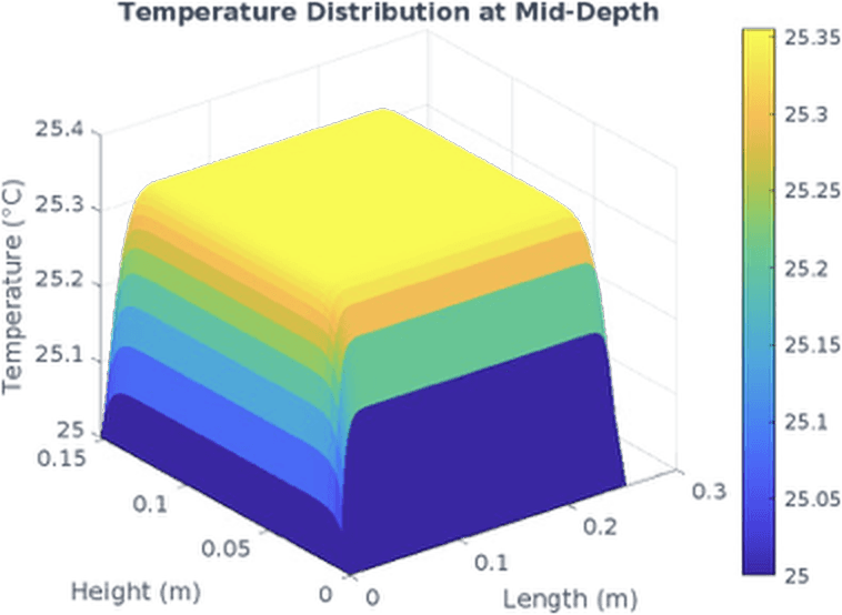
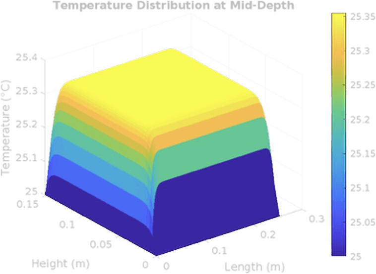
The MATLAB implementation converged after 11,762 iterations under the same numerical tolerance and physical assumptions. Despite a nearly identical iteration count, the total execution time was approximately 81 seconds on the same hardware platform, representing a substantial performance advantage relative to the Python implementation.

The steady-state temperature distribution exhibits the same qualitative features observed in the Python results, including a temperature gradient from the coolant inlet at the bottom to the outlet at the top of the battery. Lower temperatures are observed near the bottom and lateral boundaries due to the imposed coolant profile and convective heat transfer to the ambient environment. The close agreement in temperature patterns between the two implementations indicates numerical consistency, while the large difference in runtime highlights significant differences in computational efficiency.

MATLAB surface plot of the same mid-depth temperature field, ranging from 25.0 to 25.35 °C — Figure 3. Steady-state temperature at mid-depth of the battery, from the MATLAB solver.

Discussion and Conclusions

This study demonstrates a substantial performance difference between MATLAB and Python for solving a three-dimensional transient heat diffusion problem under identical physical assumptions, numerical methods, and hardware constraints. Although both environments are interpreted and support optimized numerical computation, MATLAB achieved an approximately 40× reduction in execution time relative to the Python implementation while converging in a nearly identical number of iterations. This result suggests that MATLAB’s tightly integrated numerical libraries, execution model, and Just-In-Time optimization can provide significant performance advantages for certain PDE-based simulations.

It is important to note that this performance advantage should not be assumed to generalize across all classes of partial differential equations or numerical methods. The observed speedup is problem-dependent and influenced by factors such as discretization strategy, solver implementation, memory access patterns, and library-level optimizations. Further investigation, including comparisons with alternative Python runtimes and optimized numerical backends, would be required to assess the broader applicability of these results.

Despite the observed differences in execution time, a central outcome of this study is that computationally intensive three-dimensional transient simulations can be performed effectively on standard consumer hardware. Both implementations successfully converged on a modern laptop, indicating that meaningful PDE-based engineering analysis does not inherently require specialized or high-performance computing resources. This finding highlights the accessibility of numerical simulation for engineers and reinforces the importance of selecting computational tools based on problem characteristics, performance requirements, and available resources rather than perceived hardware limitations.